This week's topics covered time-series analysis and smoothing techniques of time-series data.

---

Question # 1 : Apply the procedures outlined in the assignment details to the Tampa weather data and create a report involving hypotheses.

Null hypothesis
H₀: The average annual precipitation of the data set shows a linear upward trend.

Alternative hypothesis
H₁: The average annual precipitation of the data set does not show a linear upward trend.

  #Install library to handle .xlsx files
  > install.packages("readxl")
  > library(readxl)

  #Import provided data
  > tampaweather <- read_excel("tampadata.xlsx", sheet=1)

  #Separate precipitation column for analysis
  #Values for year will be input via time series object
  > tamparain <- tampaweather[,9]

  #Convert data to time series object
  > tampaprecip.ts <- ts(tamparain, freq=1, start=1900)
  Warning message:
  In data.matrix(data) : NAs introduced by coercion

  #Account for values of 'NA'
  > is.na(tampaprecip.ts) <- 0

  #Print time series
  > print(tampaprecip.ts)
  Time Series:
  Start = 1900
  End = 2017
  Frequency = 1
         Precip
    [1,]   1.06
    [2,]   1.45
    [3,]   0.60
    [4,]   1.27
    [5,]   2.51
    [6,]   1.64
    [7,]   1.91
    [8,]   4.68
    [9,]   1.06
   [10,]   2.50
   [11,]   2.48
   [12,]   1.30
   [13,]   1.69
   [14,]   3.02
   [15,]   2.23
   [16,]   1.09
   [17,]   4.03
   [18,]   0.92
   [19,]   0.91
   [20,]   1.40
   [21,]   2.16
   [22,]   0.45
   [23,]   1.23
   [24,]   1.66
   [25,]   2.10
   [26,]   0.75
   [27,]   1.66
   [28,]   1.53
   [29,]   1.41
   [30,]   3.43
   [31,]   3.08
   [32,]   1.53
   [33,]   3.97
   [34,]   0.91
   [35,]   0.93
   [36,]   1.67
   [37,]   1.26
   [38,]   2.78
   [39,]   1.04
   [40,]   2.22
   [41,]   1.71
   [42,]   1.66
   [43,]   2.12
   [44,]   2.40
   [45,]   1.50
   [46,]   0.52
   [47,]   1.56
   [48,]   1.68
   [49,]   1.25
   [50,]   2.96
   [51,]   4.44
   [52,]   1.19
   [53,]   3.68
   [54,]   1.86
   [55,]   1.59
   [56,]     NA
   [57,]   0.88
   [58,]   1.74
   [59,]   0.60
   [60,]   2.77
   [61,]   2.79
   [62,]   0.18
   [63,]   1.48
   [64,]   0.48
   [65,]   1.45
   [66,]   3.08
   [67,]   0.41
   [68,]   2.49
   [69,]   1.69
   [70,]   2.75
   [71,]   1.25
   [72,]   0.83
   [73,]   1.14
   [74,]   1.24
   [75,]   2.37
   [76,]   2.99
   [77,]   1.79
   [78,]   1.10
   [79,]   3.51
   [80,]   2.25
   [81,]   0.94
   [82,]   0.62
   [83,]   2.96
   [84,]   1.23
   [85,]   0.96
   [86,]   2.90
   [87,]   1.25
   [88,]   2.35
   [89,]   1.37
   [90,]   2.11
   [91,]   2.03
   [92,]   1.74
   [93,]   3.00
   [94,]   4.37
   [95,]   3.28
   [96,]   3.66
   [97,]   2.34
   [98,]   2.70
   [99,]   3.32
  [100,]   5.01
  [101,]   1.96
  [102,]   1.32
  [103,]   3.41
  [104,]   0.93
  [105,]   2.22
  [106,]   4.46
  [107,]   4.32
  [108,]   4.31
  [109,]   4.26
  [110,]   2.16
  [111,]   1.10
  [112,]   2.07
  [113,]   3.06
  [114,]   3.81
  [115,]   3.48
  [116,]   1.81
  [117,]   1.80
  [118,]   4.00


  #Give the chart file a name
  > png(file = "tampaprecip.png")

  #Plot a graph of the time series
  > plot(tampaprecip.ts, asp=5, main = "Tampa Rain
        from 1900 - 2017")

  #Save the file
  > dev.off()

          

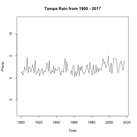
Based on the results from the time series visualization, there appears to be a slight linear trend in the upward direction. Therefore, we accept the null hypothesis. It is worth noting that a forecast line would smooth the line graph and more clearly show if a trend is apparent, however, this was unable to be applied to the time series.

Note: I attempted to add a forecast line using exponential smoothing via the HoltWinters function per the Avril Coghlan text, however I kept receving an error saying I had values of NA even though I had removed them. I was unable to resolve this error.

  > precipforecasts <- HoltWinters(tampaprecip.ts,
      beta=FALSE, gamma=FALSE)
  Error in hw(p, beta, gamma) : NA/NaN/Inf in
    foreign function call (arg 1)

---